Any stock trading strategy is confronted with what will trigger a trade. It is the same problem as a discretionary trader or investor would face. Except that in an automated trading system, all you can use will be based on retrieved data, programmed assignments, equations and conditionals. There are no gut feelings or emotions, only quantifiable "stuff" you can assign, scale or select with an $\text {if then else}$.
The portfolio payoff matrix equation was set at: $$A(t) = A_0\, + \displaystyle{\sum_{i=1}^n }(H\,.^*\Delta_i{P}) = A_0 + n \cdot \bar x $$
with inventory matrix: $H = B \,.^- S$, where the $B$uy matrix adds shares to the inventory and the $S$ell matrix removes them. The main interest is in the payoff matrix: the total profit or loss, which by the above, was reduced to just two numbers: $\,n \cdot \bar x$. Whatever you do trading can be described using those two numbers. One of them $n$ is a counter.
One needs a decision to buy, add to inventory, and to sell shares from it. This decision element could be seen as: $d_{i,\,j}\, \in \lbrack 0, 1 \rbrack$, a simple on and off switch. As a decision matrix $D$, it can affect the entire payoff matrix: ${\sum_{i=1}^n }(H \,.^*D \,.^*\Delta{P})$ since the buy matrix would depend on this decision process: $B\,.^*D$. Even putting a decision process on the table raises questions. One needs to consider that the decision process could and can be different that you want to buy shares or sell some from inventory. Therefore, you deduce you need 2 decision matrices: $D_b\,, \,D_s$, one triggering buys and the other to allow selling from inventory.
A decision is not enough, it might provide the yes or no on a trade, but it says nothing as to how much should be traded in or out. You need another matrix to determine the quantity $q_{i,\,j}\,$ to be traded. So, for the $B$uy matrix this would translate to: $B_b\,.^*D_b\,.^*Q_b$. We can simplify the problem by making the $B$uy matrix the holder of the traded quantities and control the conditionals from the outside.
But, there is still missing one element: an enhancer, a scaler, a kind of emphasis added on certain scenarios: $e_{i,\,j}\,$. Then the enhancer matrix $E$ could scale up or down the quantity matrix $\,Q \,$ depending on analyzed factors surrounding the decision matrix.
We could have a payoff matrix looking like this: ${\sum_{i=1}^n }((H = (B\,.^*D_b\,.^*Q_b\,.^*E)\,\,{.^-}\, (S\,.^*D_s\,.^*Q_s))\,.^*\Delta{P})$ with its decision process in place with a scaling function to adjust quantities to whatever level dictated by the program as long as trades are feasible and marketable. Or, simply use: ${\sum_{i=1}^n }(H \,.^*\Delta{P})$, and control everything from within $H$.
If you have a small inventory on hand for some highly liquid stock, the selling part should be relatively easy to execute. It becomes more difficult and in itself a problem when $n$ becomes large. Like, you can not flip a million trades every minute! The problem should be addressed when considering a long term trading strategy since you want $n$ to be large, as in: $\,n \cdot \bar x$.
It is a question of equilibrium. If you want more, you will have to push for more. Grab more of what is out there.
On the other hand, you are operating under uncertainty, under risk, and if you push too much, your house of cards might crumble. But, there is a lot of room before reaching any disastrous limits. You can program your system to never even get close to them. And if that is what you want, then you should figure out, beforehand, what those limits are in order to never cross the line.
The fact that you will be operating under uncertainly makes predicting difficult. Nonetheless, you do have decades of statistical data on how the market behaved. It can answer general questions as long as you are looking at this past data. But when it comes to the future, a lot of the data becomes useless. The future is a new game, a new frontier, all stocks might behave differently from their past. New stock price series will have their own unique signatures, their singular path leading them either to higher prices or oblivion.
But still, it is the trading universe in which you have to extract your profits. The what you do or how you do it is your own thing. There are other participants in the game. Consider them as just being there to facilitate your trading in and out of positions.
You will have your own game, let them have theirs. I am tempted to say: the "game" at hand is your trading strategy $H$.
The expression: $\, n \cdot \bar x \,$ is the output of a trading strategy. It could be broken down into two parts:
$$ \, n \cdot \bar x \, = (n - \lambda) \cdot \bar x_{_+} + \, \lambda \cdot \bar x_{_-} \quad \quad \text {with}\,\, \lambda\, \text {, the number of losing trades:}\,\, 0 \leq \,\lambda \, \leq n$$and where $\, \bar x_{_-} \, $ and $\,\, \bar x_{_+}\, $ represent respectively the average loss per losing trade, and the average profit per trade from winning trades. It enables the study of generated profits and losses separately. The average profit per trade $\bar x$ could also be expressed as: $\displaystyle \bar x = \,\,\bar x_{_+}\cdot (1-\frac {\lambda}{n}) + \lambda \cdot \bar x_{_-}$. Just based on that equation, you want $\,\lambda\,$ to be only a small fraction of total trades.
It follows that $\,\bar x\,$ is between the two extremes: $\,\bar x_{_-} \leq \,\bar x \, \leq \, \bar x_{_+}$ . The limit as $\lambda \,$ tends to zero is $\bar x_{_+}$ as in: $\displaystyle \lim_{\lambda\, \rightarrow \,0}n \cdot \bar x=\,n \cdot \bar x_{_+}$. And conversely, as $\lambda \,$ tends to $n$, the portfolio gets filled with losing trades: $\displaystyle \lim_{\lambda\, \rightarrow \,n}n \cdot \bar x=\,n \cdot \bar x_{_-}$.
You want $\,\bar x \,$, the average of it all to be positive. And therefore, there is a balance to be reached. But, nothing stops anyone from reaching for: $\lambda\, \rightarrow \,0$, since going the other way: $\lambda\, \rightarrow \,n$, will get you out of the game with nothing to show for it.
http://alphapowertrading.com/images/divers/AverageWinDistribution.png
The above chart shows the average profit per trade: $\,\bar x\, $, (dark blue line). It is bell-shaped in distribution, appears Gaussian but just for illustrative purposes. The actual shape has skewness, kurtosis, fat tails, bumps and other erratic shapes, all smoothed out as $n$ gets larger. But still, this chaotic bell-shaped curve has a mean $\mu$ and something close to a standard deviation $\sigma$. So, let's say we have a quasi bell-shaped curve and keep it fuzzy looking.
The object of the trading game will be to shift: $\,\,\bar x_µ\, $ to $\,\, \bar x_{µ_+}$. However, just the shifting is not enough. The task is to also improve on $\, n \cdot \bar x \,$, and this will require some added effort. Shifting the mean to the right helps, but we need to increase the curve's density. This is accomplished by the green bell-shaped curve. It will require that $n$ be part of the deal.
The response, the green curve, increased the average profit per trade as well as increased the number of profitable trades. And that is what will start to enable the function: $(1+g(t))^{t-1}$, as discussed in a prior notebook.
The cumulative distribution function of the green line has been shifted to the right resulting in an increase average profit per trade. Any trading mechanism enabling such a feature should be more than welcomed in any trading strategy. It implies that as time goes by, one is ready to take more trades and requesting a higher profit per trade before releasing part of its inventory holdings. One could have a gradual shift from $\,\,\bar x_µ\, $ to $\,\, \bar x_{µ_+}$. Or, have the program jump to the desired level and progress further from there. This is subject to the trading methods used. Any shifting to the right, ever further than what is shown in chart $\# 1$ is desirable. It can be scaled by $n$, $q$ and $\Delta p$.
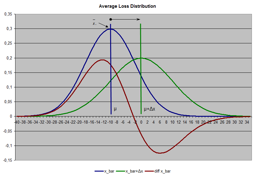
http://alphapowertrading.com/images/divers/AverageLossDistribution.png
The average loss distribution chart above has a different story to tell. Here $\,\mu\,$ the average loss per trade is moved from $\,\,\bar x_{µ_-} $ to $\,\,\bar x_µ \, $, also shifting it to the right to get the green curve.
This will reduce the average loss per trade. Overall, it should help the trading strategy by eliminating some of its losing trades. Here too, there is added work to be done to reduce the losses footprint, meaning doing less losing trades in order to generate the lower density green line.
The green curve has a lower average lost per trade on a smaller number of trades, thereby helping in the overall portfolio performance department. The portfolio as a whole is making more money simply because it is losing less than it should have: $\,\bar x_{µ_-}$.
Both charts above look about the same, but the shifting to the right of both these curves can have quite an impact on a trading strategy over the long haul. It is not just one trade that we want to affect, it is all of them, from start to finish. Even those that have not been traded yet since the program will treat them as it has treated its inventory in the past.
You are changing the rules of the game, not from outside since you know you can not change anything there, but from inside by playing "a" game were you set up the rules of engagement on your own terms. For you, it will be playing according to your rules, a game you know you will win over the long haul.
You won't win all trades, you know that. You won't predict the market's outcome on a daily basis, you know that. You won't have the ultimate trading strategy out there, but, you know that too. However, what you will have is a different understanding of the game: your own. Where you do what you think is more beneficial to you over the long term. Not by accepting to trade with a trading strategy that will fail over time, but with one that can survive for decades.
It changes the vision you have of your portfolio. From a Markowitz rebalancing act from period to period optimization problem to one of multi-period multi-asset long term assessments of trading procedures under uncertainty.
What a simulation over past data shows is: how your trading strategy would have behaved, how profitable it could have been over the selected stocks using the available data. A kind of proof of concept thing. It still won't predict the future. But, it will say: had you done this or that over the last 20$^+$ years over those stocks, it would have generated this or that total profit or loss.
You know the future will be different. It won't give the same numbers, but I do think that, having done the simulations does increase your odds going forward. Not doing the simulations, or not wanting to do the simulations, is only saying that you are ready to go at it blind without any evidence that what you have in mind could actually be profitable over the long term. I don't see losing slowly, depleting one's trading account as a viable option.
There is only one place where you don't really need to test a trading strategy. You don't even need a computer to do the job. And that is in a long term discretionary investment strategy where proof of concept has already been demonstrated time and time again. Trading a Buffett like investment strategy over some 50 years, you are bound to be profitable, almost as a matter of fact, no matter what.
But short term trading to last is another game altogether. You need to demonstrate in some way or other that the concepts you want to put on the table are justifiable. And this can only be done by showing some statistical evidence based on those trading concepts. It is always your choice. But you should realized that first, you have to show to yourself that what you think as a trading methodology makes sense, that it could be realizable, be executable in the market place, be sustainable and generate more than just buying index funds. Otherwise, why do all this?
In my strategy designs, I try to implement what's in chart $\# 1$ and $\# 2$. I do go a little bit further since I do want the payoff matrix to act as: $$A(t) = A_0\, + \displaystyle{\sum_{i=1}^n }(H \cdot (1+g(t))^{t-1}\,.^*\Delta{P}) $$ by shifting $\,\,\bar x_{µ_-} \, $ to $\,\,\bar x_µ \, $ in chart $\# 2$, while pushing $\,\,\bar x_µ\, $ to $\,\, \bar x_{µ_+}\, $ in $\# 1$. Anyone can go beyond what is shown in chart $\# 1$. The objective is to increase the density under the green curve as well as move its mean $\mu$ to the right as much as you possibly can. Increasing $\, n \cdot \bar x \,$ using its two components, will translate into a higher long term portfolio CAGR.
The technique used to implement the above is secondary. There are a multitude of procedures that can help shift both dark blue curves to the right in the above charts, and transform them into their respective restructured green curves.
For instance, one of my programs uses what I call delayed gratification to shift $\,\bar x_µ \,$ to the right, thereby shifting the whole bell shaped curve to the right. I have other procedures specialized in increasing the number of trades at those levels. The result is an improved portfolio performance. It is as if because you could draw some pictures, you now were able to better see and design trading strategies to respect these curves. They also serve as an explanation for what to do. You provide a mathematical representation of what you do and its consequences.
I do not think it matters so much the how you do it, but as long as what you do will shift those $\,\bar x \,$ curves to the right, your portfolio performance should improve, not only for the short term, but for the long term as well. This is the change of vision. You are not looking to affect a trade here and there, or trying to exploit some anomaly somewhere on the price line, you are designing procedures that will affect the entire payoff matrix at a time. Your strategy design will have built-in procedures to make it last and thrive. And the more you will play with these procedures, the more you will find resemblance to some of Mr. Buffett's own trading methods.
My trading techniques also include the accumulation of shares over long term horizons. Part of the portfolio becomes an increasing core position in each of the traded stocks. Part or all of a stock's inventory is liquidated for either of two scenarios. One, the company is purchased and you get the merger price which is usually at a premium, or two, the company gets into trouble in which case a big red button liquidates the stock's shares long before there is real trouble like bankruptcy or fraud. You can program your trading strategy with protective countermeasures. It is a matter of choice. It is your program.
There is a stock selection process to be done for sure, but the interest should be in $\,n\,$ and $\,\bar x\,$. It is on ways to detect as many $\,\Delta p\,$ as possible, since one does want $\,\Delta p\,> 0$. Any method that will get closer to that goal should be investigated.
From chart $\#$1, shifting to the right can be accomplished rather easily. Say you use a trading unit, a fixed amount per trade, and you set a profit target of say 10% which on profitable trades will give: $(n - \lambda)\cdot\bar x_{_+}$. Increasing the target to say 12% will result in: $(n - \lambda) \cdot \bar x_{_+}\cdot (1+0.02) $. With $\bar x_{_+} $ shifted to the right by 2%. One should note that having a percent profit target renders the game linear since your average profit per trade unit is being fixed at your desired level, and here, the $n$ in $\,n\,\cdot \bar x\,$ will play a major role. How many times can you do a 12% profit target on closed trades?
The easiest way to increase $\,n\,\cdot \bar x\,$ is to provide it with more time. From Strategy Design Defects we have that $\bar x$ tends to increase, on average, over extended periods of time: $$ \,\, \bar x = \displaystyle \frac {A_0 \cdot \lbrace (1+r)^t - 1\rbrace}{n}$$ This implies, on average, $\bar x$ will shift to the right on its own, just by giving it time. Also, the value of this average profit per trade $\bar x$ will be proportional to $A_0$, the initial trading capital. For example, a bag holder will see $\bar x$, on average, grow at the same rate as the market's secular trend. It further implies that $\bar x$ can move quite far to the right on chart $\#$1 without doing anything other than wait.
My task using Quantopian will be to transform some of my programs to Python. Already part of the job is done due to the richness of the programming language. I needed vector manipulation and matrix operations, all easily done with Python. Also, a few minor attempts have been done on cloned programs where just modifying pivotal decision points increased performance considerably. So that, in a better structured environment, more suitable to my trading procedures, I should be able to do more.
See the 3-part article series entitled: Simple Stock Trading Strategy: http://alphapowertrading.com/index.php/papers/214-simple-stock-trading-i where is shown a trading strategy that already contains a framework I might need to do the job. I will probably end up using something quite different from the illustrated trading strategy, but it should be nonetheless a reasonable candidate to get reacquainted with Python programming. Since that strategy was stripped of its premises, its efficiency rating wasn't worth a dime, and it got heavily in stocks at the top of market cycles, there won't be much left from the original script after I'm finished with it. Only the structural skeleton might remain which in itself is the Quantopian default setting when requesting a new trading strategy.
Have some work to do, mostly learn Python. Exciting.
© 2016, October 2nd. Guy R. Fleury