Stock Portfolio Strategy Design¶

Every day you are told which stocks performed best and which did not. Your stock trading program can monitor all those stocks and sort them out over whatever criteria you like. One would imagine that your stock ranking system would make you concentrate on the very best performers. However, when looking at long-term portfolio results, it should raise more than some doubts on this matter since most professional stock portfolio managers do not even outperform market averages.

Comparing stock trading strategies should be made over comparables, meaning over the same duration using the same amount as initial capital. It should answer the question, is strategy $ H_k $ better than $ H_{spy} $ or not?

$\quad \quad \sum (H_k \cdot \Delta P) >, \dots, > \sum (H_{spy} \cdot \Delta P) >, \dots, > \sum (H_z \cdot \Delta P)$ ?

So, why is it that most long-term active trading strategies fail to beat the averages? Already, we expect half of those strategies should perform below averages almost by definition. But, why are there so many more?

$\quad \quad \displaystyle{ \sum (\overline{H_k} \cdot \Delta P) < \sum (H_{spy} \cdot \Delta P)}\quad $ for $k=1 $ to some gazillion strategies out there.

It is a legitimate question since you will be faced with the same problem going forward. Will you be able to outperform the averages? Are you looking for this ultimate strategy $ H_{k=5654458935527819358914774892147856} $? Or will this number require up to some 75 more digits...

We have no way of knowing how many trading strategies or which ones can or will surpass the average benchmark over the long term. But, we do know that over the past, some 75$ \% $, maybe even more, have not exceeded long-term market averages. This leaves some 25$ \% $ or less that have satisfied the condition of outperforming the averages. It is from that lot that we should learn what to do to improve on our own trading strategies.

We can still look at the strategies that failed in order not to follow in their footsteps. Imitating strategies that underperform over the long term is not the best starting point. It can only lead to underperforming the averages even more.

We need to study and learn from the higher class of trading strategies and know why they outperformed. If we cannot understand the rationale behind such trading strategies or if none is given, then how could we ever duplicate their performance or even enhance them?

We have this big blob of price data, the recorded price matrix $ \mathsf{P} $ for all the listed stocks. We can reduce it to a desirable portfolio size by selecting as many columns (stocks) and rows (days) as we like, need or want. Each price is totally described by its place in the price matrix $ p_{d,j} $. And what you want to do is find common grounds in all this data that might show some predictive abilities.

You have stock prices going up or down, they usually do not maintain the same value very long. So, you are faced with a game where at any one time prices are basically moving up or down. And all you have to determine is which way they are going. How hard could that be?

From the long-term outcome of professional stock portfolio managers, it does appear to be more difficult than it seems.

There is Randomness in There¶

If price predictability is low, all by itself, it would easily explain the fact that most professionals do not outperform the averages over the long term. As a direct consequence, there should be a lot of randomness in price movements. And if, or since, it is the case, then most results would tend to some expected mean which is the long-term market average return.

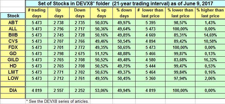
It is easy to demonstrate the near 50/50 odds of having up and down price movements. Simply count the ups and downs days over an extended period of time over a reasonable sample. The expectation is that you will get, on average, something like 51/49 or 52/48 depending on the chosen sample. The chart below does illustrate this clearly.

With those numbers, we have to accept that there is a lot of randomness in the making of those price series. It takes 100 trades to be ahead 2 or 4 trades respectively. With 1000 trades, you should be ahead by 20 or 40 trades. But, you will have to execute those 1000 trades to achieve those results. That is a 2$ \% $ or a 4$ \% $ of trades taken that will account for most of your generated profits. This says that the top 50 trades out of the 1000 taken will be responsible for most if not all your profits. And that 950 trades out of those 1000 could have been throwaways. Certainly, the 48% of trades you lost (480 trades), if they could have been scraped would definitely have helped your cause, profitwise.

The problem you encounter is that you do not know which one is which, and thus, the notion of a high degree of randomness. Fortunately, it is only a high degree of randomness and not something that is totally random because there only luck could make you win the game.

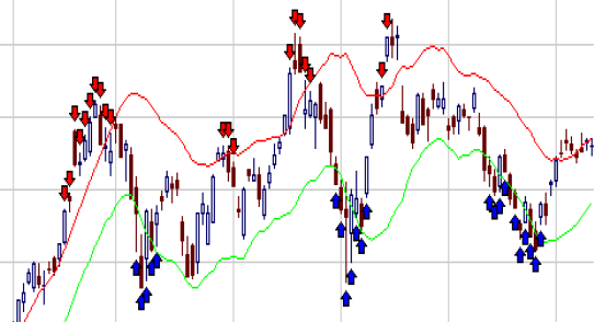
Here is an interesting AAPL chart snippet (taken from my 2012 Presentation). It makes that presentation something like a 7-year walk-forward with totally out-of-sample data. The hit rate on that one is very high. It is also the kind of chart we do not see on Quantopian. It was done to answer the question: are the trades executed at reasonable places in the price cycles? A simple look at the chart can answer that question.

The chart displays the strategy's trading behavior with its distributed buys (blue arrows) and sells (red arrows) as the price swings up and down. On most swings, some shares are sold near tops and bought near bottoms. The chart is not displayed as a probabilistic technique, but to show some other properties.

One, there was no prediction made in handling the trades, none whatsoever. The program does not know what a top or bottom is or even has a notion of mean-reversal. Nonetheless, it trades as if it knew something and does make trading profits.

Second, entries and exits were performed according to the outcome of time-biased random functions. There are no factors here, no fundamental data, and no technical indicators. It operates on price alone. It does, however, have the notion of delayed gratification. An exit could be delayed following some other random functions giving a trade a time-measured probabilistic exit. Meaning that a trade could have exceeded its exit criteria but its exit could still be ignored until a later date for no other reason than it was not its lucky exit day.

Third, trades were distributed over time in an entry or exit averaging process. The mindset here is to average out the average price near swing tops or bottoms. The program does not know where the tops or bottoms are but nonetheless its trade positioning process will make it have an average price near those swing tops and bottoms.

Forth, the whole strategy goes on the premise of: accumulate shares over the long term and trade over the process (this is DEVX03 that gradually morphed over the years into its latest iteration DEVX10). The above chart depicts the trading process but does not show the accumulation process itself even if it is there. To accumulate shares requires that as time progresses, the stock inventory increases by some measure as prices rise.

Here, the proceeds of all sales, including all the profits, are reinvested in buying more shares going forward. And this share accumulation, as well as the accumulated trading profits, will be reflected in the strategy's overall long-term CAGR performance. It is all explained in the above-cited 2012 presentation.

Trading Methodology¶

The trading methodology itself accounts for everything. It is the method of play that determined how to make the strategy more productive. Just looking at the chart, we have to consider that there was a lot of day to day randomness in those price swings. Yet, without predicting, without technical or fundamental indicators, the strategy managed to prosper over its 5.8-year simulation (1,500 trading days).

Since that 2012 presentation, AAPL has quadrupled in price and all along the strategy would have accumulated even more shares and evidently would have profited from its trading operations even more. Whereas the AMZN example would have seen its price go from 176.27 to over 1,800 today. All the while accumulating more and more shares as the shares went up in price. The strategy profited from the rise in price with a rising inventory and profited from all the trading activity.

The strategy is based on old methods and does show that it can outperform the averages: $\sum (H_k \cdot \Delta P) \gg \sum (H_{spy} \cdot \Delta P) $. The major force behind strategy $ H_k $ is time. As simple as that. It waits for its trade profit. It was easy to determine some seven years ago that AAPL and AMZN would prosper going forward. We can say the same thing today for the years to come. What that program will do is continue to accumulate shares for the long term and trade over the process, and thereby continue to outperform the averages.

Time is a critical factor in a trading strategy. For instance, to the question: if you waited to exit a trade, would you make a profit? To illustrate this, I made the chart below where the red lines would have shown that having picked any of the 427 days shown you would have had a losing trade. On the other side, a green line showed that picking that trading day out of the 427 days, it would have ended with a profit. As can be seen, all 427 trading days could have ended with a profit. Moreover, you could have had multiple attempts at making a profit during the trading interval. Simply picking any one day would have resulted in profits just for having waited for that profit. Nothing fancy needed for this except giving the trade some time.

In the end, we all have to make choices. Some are easier than others. But one thing is sure, it will all be in your trading strategy $ H_k $ and what you designed it to do.

Do do the best you can since the above does say it can be done.